【Python入門】ベクトルの可視化｜Matplotlibで描画する

「ベクトル」は、Pythonで容易に可視化することができます。

本記事では、Pythonを使用したベクトルの可視化方法について、詳しくご説明します。

levtech-ad

＼業界最大級の案件数！／

レバテックフリーランス詳細はコチラ＞＞

ベクトルの可視化

Matplotlibを使用したベクトルの可視化（描画）方法について、ご説明します。

matplotlib.axes.Axes.quiver()

Matplotlibのmatplotlib.axes.Axes.quiver()関数を使用すると、二次元ベクトル場にベクトルを描画することができます。

引数には、ベクトルの始点の\(x\)座標、始点の\(y\)座標、ベクトルの\(x\)成分（\(\Delta x\)）、ベクトルの\(y\)成分（\(\Delta y\)）の順で指定します。

以下に使用例をご紹介します。

#input
import numpy as np
import matplotlib.pyplot as plt

fig = plt.figure(figsize = (5, 5))
ax = fig.add_subplot(111)

ax.grid()

ax.set_xlabel("x", fontsize = 14)
ax.set_ylabel("y", fontsize = 14)

ax.set_xlim(-6, 6)
ax.set_ylim(-6, 6)

ax.axhline(0, color = "black")
ax.axvline(0, color = "black")

ax.quiver(-3, -3, 7, 5, color = "red",
          angles = 'xy', scale_units = 'xy', scale = 1)

ax.text(-5.2, -3, "[-3, -3]", color = "red", size = 15)
ax.text(4, 2, "[4, 2]", color = "red", size = 15)

plt.show()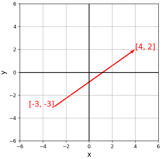

ベクトルの太さは「width」で指定することができます。

ベクトルを１本増やし、widthを指定して少し太くした例を以下にご紹介します。

#input
import numpy as np
import matplotlib.pyplot as plt

fig = plt.figure(figsize = (5, 5))
ax = fig.add_subplot(111)

ax.grid()

ax.set_xlabel("x", fontsize = 14)
ax.set_ylabel("y", fontsize = 14)

ax.set_xlim(-6, 6)
ax.set_ylim(-6, 6)

ax.axhline(0, color = "black")
ax.axvline(0, color = "black")

ax.quiver(-3, -3, 7, 5, color = "red", width=0.02,
          angles = 'xy', scale_units = 'xy', scale = 1)

ax.quiver(-3, 3, 7, -5, color = "blue", width=0.02,
          angles = 'xy', scale_units = 'xy', scale = 1)

ax.text(-5.2, -3, "[-3, -3]", color = "red", size = 15)
ax.text(4, 2, "[4, 2]", color = "red", size = 15)
ax.text(-5.2, 3, "[-3, 3]", color = "red", size = 15)
ax.text(4, -2, "[4, -2]", color = "red", size = 15)

plt.show()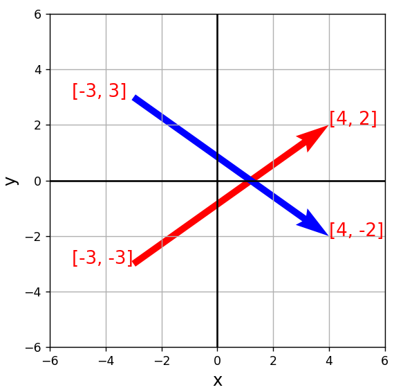

Axes.quiver()関数は各ベクトルの始点や成分を指定する必要がありますので、複数のベクトルを描画する場合には、手間が多いです。

そこで、より簡易的にベクトルを描画できるような関数を以下に実装してみます。

visual_vector()

簡易的にベクトルを描画できる関数として、visual_vector()を実装してみます。

#input
def coordinate(axes, range_x, range_y, grid = True,
               xyline = True, xlabel = "x", ylabel = "y"):
    axes.set_xlabel(xlabel, fontsize = 14)
    axes.set_ylabel(ylabel, fontsize = 14)
    axes.set_xlim(range_x[0], range_x[1])
    axes.set_ylim(range_y[0], range_y[1])
    if grid == True:
        axes.grid()
    if xyline == True:
        axes.axhline(0, color = "black")
        axes.axvline(0, color = "black")

def visual_vector(axes, loc, vector, color = "red"):
    axes.quiver(loc[0], loc[1],
              vector[0], vector[1], color = color, width=0.01,
              angles = 'xy', scale_units = 'xy', scale = 1)

上記実装した関数を使用して、ベクトルを描画してみます。

#input
import numpy as np
import matplotlib.pyplot as plt
fig = plt.figure(figsize = (5, 5))
ax = fig.add_subplot(111)

coordinate(ax, [-3, 3], [-3, 3])

v1 = np.array([2, -4])
v2 = np.array([2, 4])

# [-2,2]を始点にv1を描画
visual_vector(ax, [-2, 2], v1, "tomato")

# [0,-2]の終点を始点にv2を描画
visual_vector(ax, [0,-2], v2, "aqua")

# [-2,2]を始点にv1+v2を描画
visual_vector(ax, [-2, 2], v1 + v2, "lime")

plt.show()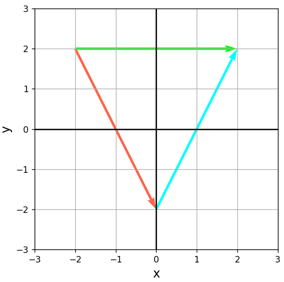

より簡易的にベクトルを描画することができました。

次に、上記関数を3次元に拡張してみます。

visual_vector_3d()

3次元拡張版として、visual_vector_3d()を実装してみます。

#input
def coordinate_3d(axes, range_x, range_y, range_z, grid = True):
    axes.set_xlabel("x", fontsize = 14)
    axes.set_ylabel("y", fontsize = 14)
    axes.set_zlabel("z", fontsize = 14)
    axes.set_xlim(range_x[0], range_x[1])
    axes.set_ylim(range_y[0], range_y[1])
    axes.set_zlim(range_z[0], range_z[1])
    if grid == True:
        axes.grid()

def visual_vector_3d(axes, loc, vector, color = "red"):
    axes.quiver(loc[0], loc[1], loc[2],
              vector[0], vector[1], vector[2],
              color = color, lw=3)

#input
import numpy as np
import matplotlib.pyplot as plt

fig = plt.figure(figsize = (6, 6))
ax = fig.add_subplot(111, projection='3d')

# 3D座標を設定
coordinate_3d(ax, [-10, 10], [-10, 10], [0, 10], grid = True)

# 始点を設定
o = [0, 0, 0]

# 3Dベクトルを定義
v1 = np.array([-7, -7, 7])
v2 = np.array([-7,  7, 7])
v3 = np.array([ 7, -7, 7])
v4 = np.array([ 7,  7, 7])

# 3Dベクトルを配置
visual_vector_3d(ax, o, v1, "red")
visual_vector_3d(ax, o, v2, "blue")
visual_vector_3d(ax, o, v3, "green")
visual_vector_3d(ax, o, v4, "magenta")
plt.show()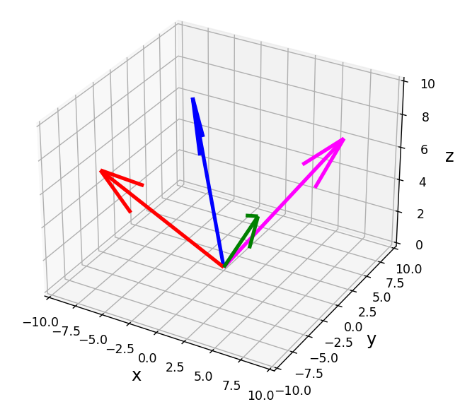

まとめ

この記事では、Pythonを使用したベクトルの可視化方法について、ご説明しました。

本記事を参考に、ぜひ試してみて下さい。

参考

Python学習用おすすめ教材

Pythonの基本を学びたい方向け

統計学基礎を学びたい方向け

Pythonの統計解析を学びたい方向け

おすすめプログラミングスクール

テックアカデミーの無料体験